

Consumer Behaviour = पसंद (preferences) + क्रय क्षमता (budget) + सबसे अच्छा उपलब्ध चुनाव (optimal choice). UGC NET Economics Unit 1 के इस topic और PGT Economics के संबंधित concepts के revision के लिए: पहले core notes पढ़ें, फिर जरूरत पर “NET extension” खोलें। सभी graphs, numericals और MCQs मौलिक illustrations हैं।
Focused topic guide: consumer choice under certainty, demand and selected mathematical tools; not the full NET syllabus. PGT syllabi vary by recruiting body. Confusion points are conceptual traps, not measured PYQ-frequency claims. Sources and syllabus.
1. Theory–Economist–Year–Work: matching table
वर्ष संबंधित मूल प्रकाशन का है। Theory का विकास कई लोगों ने किया; “introduced”, “developed” और “popularised” को एक attribution न मानें। Journal article के लिए काल्पनिक book का नाम नहीं दिया गया है।
| Contribution | Economist · year | Book or article | Exam cue |
|---|---|---|---|
| Diminishing MU; allocation across uses (Gossen’s first/second laws) | H. H. Gossen · 1854 | Entwickelung der Gesetze des menschlichen Verkehrs, und der daraus fliessenden Regeln für menschliches Handeln (book) [H1] | First: diminishing MU; second: equi-marginal allocation. |
| Marginal utility approach | W. S. Jevons · 1871 | The Theory of Political Economy (book) [H1] | Important marginalist, not the sole originator. |
| Indifference-curve geometry | F. Y. Edgeworth · 1881 | Mathematical Psychics: An Essay on the Application of Mathematics to the Moral Sciences (book) [H2] | Early IC device; Pareto developed preference analysis. |
| Marshallian demand/utility exposition; consumer surplus | Alfred Marshall · 1890 | Principles of Economics (first edition; book) [H3] | Gossen preceded Marshall; later editions have later dates. |
| Ordinal preference foundation | Vilfredo Pareto · 1906 / 1909 | Manuale di economia politica (Italian, 1906); Manuel d’économie politique (French revision, 1909) [H4] | Different editions, not contradictory dates. |
| Price-effect decomposition | Eugen Slutsky · 1915 | “Sulla teoria del bilancio del consumatore”, Giornale degli Economisti e Rivista di Statistica (article) [H5] | Old bundle stays affordable. |
| Modern ordinal demand / IC development | J. R. Hicks & R. G. D. Allen · 1934 | “A Reconsideration of the Theory of Value”, Parts I & II, Economica (articles) [H6] | 1934 = joint articles, not Value and Capital. |
| Systematic ordinal consumer-choice exposition | J. R. Hicks · 1939 | Value and Capital (book) [H4] | 1939 = Hicks’s book. |
| Revealed preference | Paul A. Samuelson · 1938 | “A Note on the Pure Theory of Consumer’s Behaviour”, Economica (article) [H7] | Observed choice; WARP. |
| Stronger revealed-preference consistency | H. S. Houthakker · 1950 | “Revealed Preference and the Utility Function”, Economica (article) [H8] | SARP: rules out cycles. |
दो अतिरिक्त attributions: Engel’s law और Cobb–Douglas form
| Concept | Who / when | Work and limit |
|---|---|---|
| Food expenditure share / Engel’s law | Ernst Engel · 1857 | “Die vorherrschenden Gewerbszweige in den Gerichtsämtern mit Beziehung auf die Productions- und Consumtionsverhältnisse des Königreichs Sachsen” (article in the Saxon Statistical Bureau journal). German statistical office reprint record. |
| Cobb–Douglas functional form | Charles W. Cobb & Paul H. Douglas · 1928 | “A Theory of Production”, American Economic Review (article). Original paper. यह production contribution था; हमारे examples में उसी form को utility के लिए उपयोग किया गया है। इसे original 1928 consumer-utility theory न लिखें। |
Gossen 54 → Jevons 71 → Edgeworth 81 → Marshall 90 → Pareto 06 → Slutsky 15 → Hicks–Allen 34 → Samuelson 38 → Hicks 39 → Houthakker 50. पहले चार 1800s; बाद के छह 1900s.
Graphs पर tap/click करके बड़ा view खोलें। Labels English में और explanations Hindi + English में हैं।
2. TU, MU और Cardinal equilibrium
Utility = subjective satisfaction, नैतिक अच्छाई या usefulness का निर्णय नहीं। Cardinal model numerical utility मानता है; ordinal model bundles की ranking चाहता है।
| Q | 0 | 1 | 2 | 3 | 4 | 5 | 6 |
|---|---|---|---|---|---|---|---|
| TU | 0 | 12 | 21 | 27 | 30 | 30 | 27 |
| MU | — | 12 | 9 | 6 | 3 | 0 | −3 |

DMU: समान quality/size की लगातार इकाइयों की MU घटती है, tastes और circumstances स्थिर रखते हुए। Introductory Marshallian model में cardinal measurement, independent utilities, rational allocation और constant MU of money जैसी assumptions उपयोग होती हैं।
Several goods, interior allocation: MUx/Px = MUy/Py = λ
MUx=Px तभी जब MU money units में हो या MU of money=1 normalise हो। सामान्य उत्तर MU per rupee बराबर है, केवल MU बराबर नहीं।
3. Preferences, IC और MRS
| Assumption | Meaning / implication |
|---|---|
| Completeness | किसी भी दो bundles को compare: A≽B या B≽A (दोनों भी)। |
| Transitivity | A≽B और B≽C ⇒ A≽C; consistent ranking. |
| Continuity | छोटे changes से abrupt preference jumps नहीं; standard utility representation में मदद। |
| Monotonicity | Desirable goods में more is better; north-east higher IC better. |
| Convexity / strict convexity | Equally ranked extremes की mixtures weakly / strictly preferred; usual smooth case में diminishing MRS. |
IC: equally preferred bundles का locus। Standard ICs downward sloping, convex to origin और distinct ICs non-intersecting। Assumptions देखें—bad, neutral good या satiation में usual shape बदल सकती है।
IC slope = −MRSxy
यहाँ MRSxy अतिरिक्त X पाने के लिए छोड़ी Y की मात्रा है। MUx=6, MUy=3 ⇒ MRS=2, slope=−2। Differentiable utility और positive MUs मानें। Books में उलटी MRS convention मिल सकती है—definition और axes पहले पढ़ें।

Substitutes = straight; complements = kink; standard mixture preference = convex. Strictly increasing f(U) ranking और IC geometry बचाती है; differentiable f with f′>0 में MU ratio भी preserved है। U=XY और ln U=ln X+ln Y (X,Y>0) same preferences; MU values अलग हो सकती हैं।
4. Budget set, intercepts और changes
Line: PxX + PyY = M
X intercept = M/Px; Y intercept = M/Py; slope = −Px/Py
M=₹120, Px=₹20, Py=₹10 ⇒ Y=12−2X। Intercepts (6,0),(0,12)। (3,6) line पर; (2,4) set के अंदर; (4,6) unaffordable।
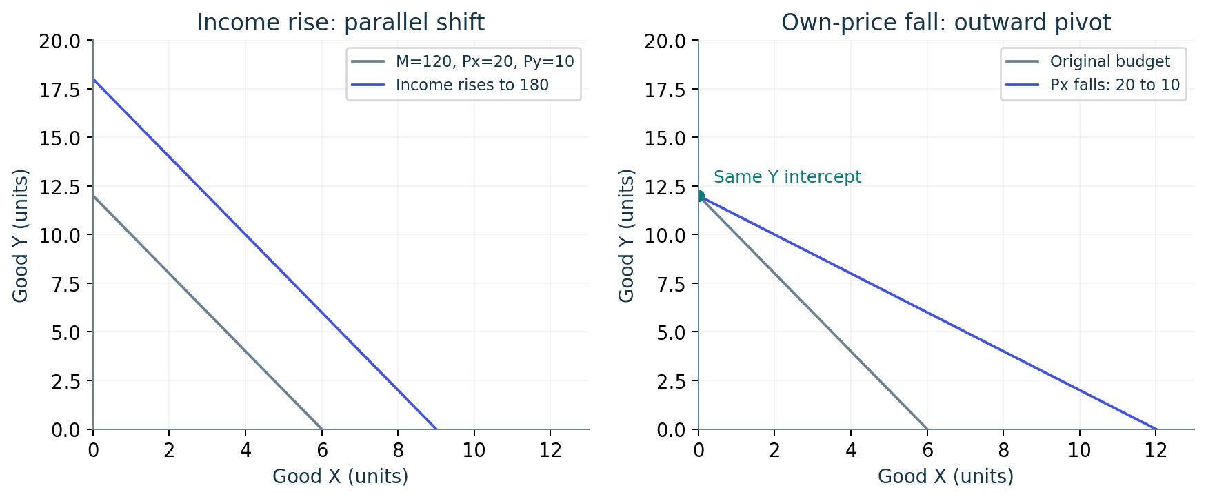
X नीचे, Y ऊपर ⇒ slope = minus “नीचे वाली वस्तु की price / ऊपर वाली वस्तु की price”। Income shifts the line; relative price changes slope.
5. Equilibrium और numerical shortcuts
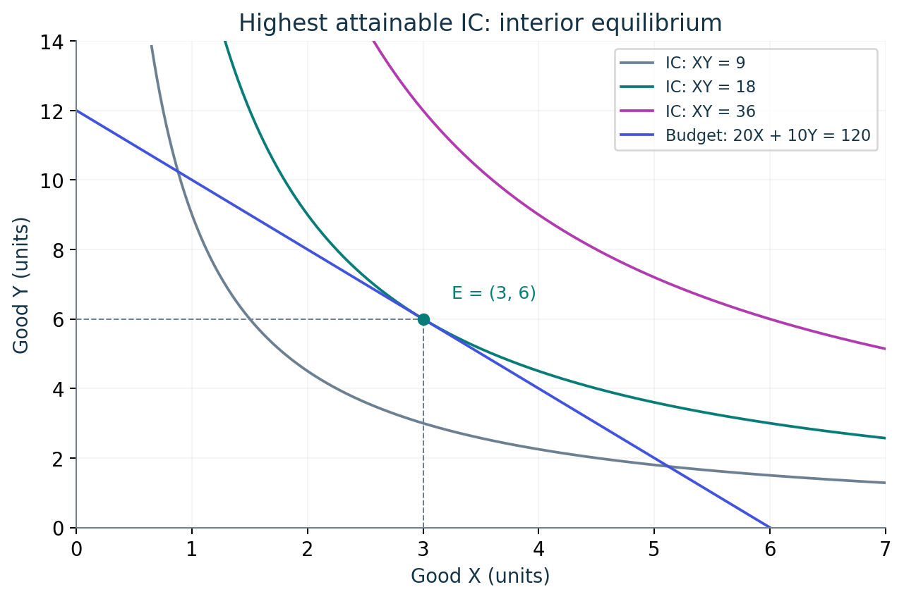
Goal: best affordable bundle। Smooth differentiable utility, positive MUs और suitable convex preferences में interior optimum:
| Utility / question | Fast method | Check / trap |
|---|---|---|
| Cobb–Douglas U=XaYb, a,b>0 | X*=aM/[(a+b)Px]; Y*=bM/[(a+b)Py]. U=XY: half income on each. | Exponents need not sum to 1; divide by a+b. Here (3,6). |
| Substitutes U=aX+bY | Compare a/Px, b/Py; spend on larger ratio. | Equal ratios: all budget-line bundles optimal. U=2X+Y, prices 3,2 ⇒ choose X. |
| Complements U=min(aX,bY) | Kink aX=bY, plus budget. X*=bM/(bPx+aPy); Y*=aM/(bPx+aPy). | min(X,2Y), M=120, prices 20,10 ⇒ X=4.8,Y=2.4. Not automatically 1:1. |
| MUx=12,Px=3; MUy=16,Py=8 | Per rupee: 4 vs 2 ⇒ initially more spending towards X. | Feasible reallocation and changing MUs matter. |
Feasibility और maximum conditions check करें। Corner optimum या complements के kink पर tangency equality जरूरी नहीं। DMU और diminishing MRS अलग हैं। Convex preferences के लिए utility quasi-concavity देखें; हर ordinal utility representation का concave होना आवश्यक नहीं।
6. Price effect = SE + IE: Hicks vs Slutsky
Px घटे, M/Py fixed: X relatively cheaper; real purchasing power बढ़ती है। Own-price compensated substitution effect X की तरफ (weakly); income effect good के type पर निर्भर।
| Compensation | Constant? | Graph clue |
|---|---|---|
| Hicks | Original utility / IC | New-price slope वाली compensated line पुराने IC को tangent करती है। |
| Slutsky | Old chosen bundle affordability | New-price slope वाली line पुराने bundle से गुजरती है; नया optimum usually old IC पर नहीं। |

Numerical: U=XY; M=120; old prices (20,10); A=(3,6), U=18। New prices (10,10) ⇒ C=(6,6)। Hicks income=2√18×10≈84.85 ⇒ H=(√18,√18), SE≈1.24, IE≈1.76। Slutsky income=old bundle at new prices=10×3+10×6=90 ⇒ S=(4.5,4.5), SE=1.5, IE=1.5।
Hicks = Happiness held; Slutsky = Same old basket affordable. Finite price changes में identical effects assume न करें।
7. Normal, Inferior, Giffen: signs से solve
| Good | Income response | SE | IE | Total |
|---|---|---|---|---|
| Normal | ∂X/∂M>0 | ↑ or zero | ↑ | ↑ (regular case) |
| Inferior, non-Giffen | ∂X/∂M<0 | ↑ or zero | ↓ | ↑ if SE dominates |
| Giffen | Inferior | ↑ or zero | ↓ | ↓; opposing IE dominates |
Giffen ⇒ inferior; inferior ⇏ Giffen. Inferior quality का नाम नहीं; income response है। Giffen own-price response है। Classification context/income range पर निर्भर है। Rice/potato universally Giffen नहीं। Veblen status/price-as-signal explanation अलग mechanism है।
NET extension · differential Slutsky equation
εxx = εhxx − sxηx
h: Hicksian; ε: signed own-price elasticity; η: income elasticity; s=PxX/M. Example εh=−0.4,s=0.6,η=−1 ⇒ ε=+0.2: locally Giffen. Own compensated derivative ≤0 under standard regularity. Inferiority alone does not ensure positive ordinary own-price derivative.
8. ICC, Engel, PCC और demand
| Curve | Change / fixed? | Axes here |
|---|---|---|
| ICC: income consumption curve | Change M; prices/tastes fixed; join optimal bundles. | X–Y goods space |
| Engel | Quantity against income; prices/tastes fixed. | X horizontal, M vertical |
| PCC: price consumption curve | Change Px; M,Py,tastes fixed; join optimal bundles. | X–Y goods space |
| Ordinary demand | X against own price; money income fixed. | X horizontal, Px vertical |


Income → ICC → Engel; Price → PCC → demand. Normal η>0; necessity 0<η<1; luxury η>1; inferior η<0. Engel’s law concerns food expenditure share—share गिरने पर भी food spending बढ़ सकती है।
9. Revealed preference: affordability पहले
A चुना गया और B उसी budget में affordable था ⇒ A directly revealed preferred to B। B unaffordable था तो choice से यह inference नहीं। Samuelson 1938; Houthakker 1950: stronger consistency.
WARP: direct two-choice reversal रोकता है। SARP: direct/indirect preference chains में cycle रोकता है। Boundary ties की weak/strict inequality convention पढ़ें। WARP को हर dimension में full rationalisation की sufficient condition न मानें।
Prices (1,2): A=(4,1) chosen costs 6; B=(1,2) costs 5 ⇒ A revealed over B. Next prices (2,1): B chosen costs 4; A costs 9 ⇒ A unaffordable, no reversal established. Instead next prices (1,4): B costs 9, A costs 8 ⇒ B chosen despite cheaper A ⇒ strict reversal, WARP violated.
10. NET tools · जरूरत पर खोलें
Optimisation, λ और ordinal invariance
MUx=λPx; MUy=λPy; budget equality (interior)
FOCs give candidates; check feasible corners/kinks and maximum conditions. λ is marginal value of income in the chosen utility units; it changes under utility transformation. Increasing transformation preserves demand/MRS, not cardinal TU/MU sizes. Convex preferences concern quasi-concavity, not compulsory concavity of every utility representation. U=XY at (3,6): λ=6/20=3/10=0.3.
Duality: Marshallian–Hicksian, Roy–Shephard
| Problem | Function / demand | Fixed |
|---|---|---|
| Max U, p·x≤M | v(p,M); Marshallian x(p,M) | Money income |
| Min p·x, U(x)≥u | e(p,u); Hicksian h(p,u) | Utility target |
Shephard: hi = ∂e/∂pi
e(p,v(p,M))=M; h(p,v(p,M))=x(p,M)
Applicable differentiability, single-valued demand and non-satiation conditions assumed. Roy→ordinary; Shephard→compensated. Works: René Roy, De l’utilité: contribution à la théorie des choix (1942); Ronald W. Shephard, Cost and Production Functions (1953). Shephard’s book concerns production/cost duality; the derivative principle also applies to consumer expenditure. [H9]
Elasticity shortcuts और adding-up
Signed εxx=(∂X/∂Px)Px/X. Elementary questions often use absolute magnitude; check notation. Same straight demand slope does not mean same point elasticity.
Σ siηi=1 (budget exhaustion; differentiable demand)
εxx=−0.8,εxy=0.2 ⇒ η=0.6. Food share=0.4,ηfood=0.5; other share=0.6 ⇒ other η=4/3. Exhausted budget implies all goods cannot be inferior at the same point. Ordinary cross effects include income effects; Hicksian cross effects isolate substitution.
11. Consumer surplus: graph और limit
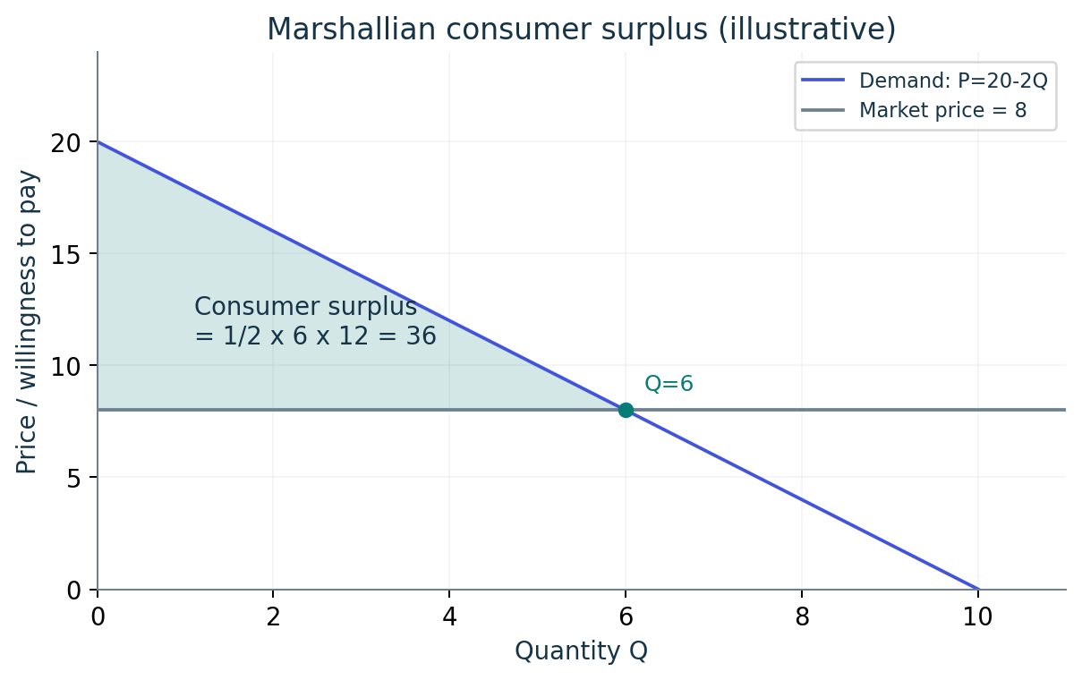
Marshallian CS = willingness to pay − actual payment; ordinary demand के नीचे, price line के ऊपर area। P=20−2Q, price=8 ⇒ Q=6; CS=½×6×12=36 money units.
NET extension · CS, CV, EV अलग हैं
Price fall p0→p1, u0=v(p0,M),u1=v(p1,M). Using positive money-value-of-gain convention:
EV=e(p0,u1)−M
CV: initial utility at new prices; EV: final utility at old prices. Textbook signs vary. Our XY price-fall example: CV≈35.15, EV≈49.71; ordinary CS gain=60 ln2≈41.59. Income effects mean CS is not generally identical to exact welfare measures; suitable quasilinear/no-income-effect cases give equality.
12. अलग Confusion Sheet · गलत option हटाएँ
| गलत shortcut | सही distinction |
|---|---|
| MU घटे ⇒ TU घटे | Positive MU तक TU बढ़ती है; zero discrete MU gives flat step. |
| Gossen=Marshall; Hicks–Allen=1939 | Gossen1854; Marshall1890; joint articles1934; Hicks book1939. |
| Ordinal means no numbers/calculus | Numbers represent ranking, cardinal happiness differences नहीं। |
| DMU automatically proves convex IC | DMU representation-dependent; diminishing MRS/convex preference अलग property। |
| Same IC ⇒ same spending | Same preference; expenditure/affordability need not match. |
| Every IC downward/strictly convex | Check desirable goods and preferences; substitutes/complements differ. |
| Equilibrium ⇒ MUx=MUy | MU/price equality, suitable interior case. |
| Any tangent point is maximum | Feasibility/maximum conditions; corners/kinks separately. |
| Hicks/Slutsky hold same thing fixed | Hicks utility; Slutsky old bundle affordability. |
| Every inferior good is Giffen | Opposing IE stronger than SE needed. |
| Compensated demand can be Giffen | Own Hicksian demand non-increasing, standard regularity. |
| ICC/PCC are Engel/demand | Goods space vs income/price axes. |
| Own price change shifts demand | Other determinants fixed ⇒ movement along; income/tastes can shift. |
| Chosen A preferred over any B | B must have been affordable then. |
| Roy→Hicksian; Shephard→Marshallian | Roy: v→x; Shephard: e→h. |
13. 2-minute revision और solving routine
- Type पहचानें: attribution, graph, numerical, assertion–reason या statements.
- Given लिखें: axes, prices, income, utility, क्या constant; finite change या derivative?
- Tool चुनें: MU difference, per-rupee ratio, budget intercept, utility shortcut, effect signs, affordability.
- Conditions: interior/corner/kink; prices positive; standard preferences; signed/absolute elasticity.
- Verify: budget में answer डालें; “always/all/only” claim की missing condition देखें।
MU positive→TU↑ · Budget slope −Px/Py · IC slope −MRS · Interior MRS=price ratio · H=utility,S=basket · Giffen⊂inferior · ICC→Engel,PCC→demand · WARP=direct reversal,SARP=cycles · Roy→x,Shephard→h.
आज graph labels बनाएं; कल formulas/attributions बिना देखे लिखें; day 3 पर गलत questions दोहराएँ। हर गलती के साथ missing condition लिखें।
Practise 30 original MCQs with explanations
Sources और scope
Checked 3 October 2026 (India). Explanations are in our own words; graphs/examples are original illustrations, not survey data or copied textbook figures.
- Official: UGC NET Economics, Unit 1 lists Theory of Consumer Behaviour. UGC syllabus index identifies applicability from June 2019 onward. Check PGT recruiting-body notifications separately.
- Concept checks: MIT OCW Consumer Theory, Alexander Wolitzky, 2015 (preferences, duality, Slutsky); MIT 14.04 readings. NCERT Introductory Microeconomics, Ch.2 is further foundation reading; its PDF could not be retrieved during this update.
- [H1] Jevons second-edition preface: Gossen1854; Jevons first edition1871. First/second laws are conventional teaching labels.
- [H2] Edgeworth original1881 text; Hicks below credits his IC device.
- [H3] Marshall Book III; first edition1890, displayed eighth edition1920.
- [H4] Hicks Value and Capital (1939), Ch.I; Pareto historical research verifies1906 Italian work; Hicks discusses1909 French work.
- [H5] Original July1915 issue: Slutsky article; also cited by Hicks.
- [H6] Original Hicks–Allen Part I, February1934, Economica; Part II followed May1934.
- [H7] Economica original February1938 issue: Samuelson.
- [H8] Economica original May1950 issue: Houthakker, pp.159–174.
- [H9] Roy1942 book catalogue; Shephard publisher record: original1953 publication. Formulas: MIT slides.
30 Original Practice MCQs · मौलिक अभ्यास प्रश्न
One correct answer per question. These are original practice questions, not official PYQs.
1. TU rises from 42 to 47 after one extra unit. What is MU? / TU 42 से 47 हो जाए तो MU कितनी होगी?
- 42
- 47
- 5
- 89
Answer and explanation
Answer: C. MU is the change in TU: 47 − 42 = 5. / MU, TU का परिवर्तन है।
2. When MU falls but remains positive, TU… / MU घट रही हो लेकिन धनात्मक हो, तो TU…
- must fall / अवश्य घटेगी
- rises at a diminishing rate / घटती दर से बढ़ेगी
- is necessarily zero / अवश्य शून्य होगी
- must stay constant / समान रहेगी
Answer and explanation
Answer: B. Positive MU adds to TU; smaller additions slow its growth. / धनात्मक MU से TU बढ़ती है, लेकिन कम दर से।
3. With X horizontal, the budget-line slope is… / X क्षैतिज अक्ष पर हो तो budget line की ढाल है…
- −Pₓ/Pᵧ
- −Pᵧ/Pₓ
- M/Pₓ
- Pₓ + Pᵧ
Answer and explanation
Answer: A. Rearrange the budget equation to Y = M/Pᵧ − (Pₓ/Pᵧ)X. / X के coefficient से ढाल मिलती है।
4. For smooth, strictly convex preferences, an interior optimum satisfies… / उपयुक्त smooth preferences वाले interior optimum में…
- MRSₓᵧ = M
- MRSₓᵧ = Pₓ/Pᵧ
- Pₓ = Pᵧ always / हमेशा
- MUₓ = 0 always / हमेशा
Answer and explanation
Answer: B. At this optimum the IC and budget line are tangent; the budget condition must also hold. / Tangency के साथ budget constraint भी पूरा होना चाहिए।
5. Which statement is correct? / कौन-सा कथन सही है?
- Every inferior good is Giffen / हर inferior वस्तु Giffen है
- No Giffen good is inferior / कोई Giffen वस्तु inferior नहीं
- Every Giffen good is inferior; the converse need not hold / हर Giffen वस्तु inferior है, विपरीत जरूरी नहीं
- Both describe luxury goods / दोनों luxury वस्तुएँ हैं
Answer and explanation
Answer: C. Giffen is a particular inferior-good case with a dominant opposing income effect. / Inferior होना अकेले पर्याप्त नहीं है।
6. When an extra unit has negative MU, TU… / अतिरिक्त इकाई की MU ऋणात्मक हो तो TU…
- increases / बढ़ती है
- does not change / नहीं बदलती
- decreases / घटती है
- becomes exactly zero / ठीक शून्य हो जाती है
Answer and explanation
Answer: C. A negative addition reduces TU; it does not necessarily reduce TU to zero. / TU घटेगी, जरूरी नहीं कि शून्य हो।
7. Income is ₹200 and X costs ₹20. With no Y purchased, maximum X is… / आय ₹200 और X की कीमत ₹20 हो तो अधिकतम X…
- 5 units / इकाइयाँ
- 10 units / इकाइयाँ
- 20 units / इकाइयाँ
- 40 units / इकाइयाँ
Answer and explanation
Answer: B. The X-intercept is M/Pₓ = 200/20 = 10. / पूरी आय X पर खर्च करने से 10 इकाइयाँ मिलेंगी।
8. Only X becomes cheaper; income and Y’s price stay fixed. The budget line… / केवल X सस्ता हो जाए तो budget line…
- shifts parallel inward / समानांतर भीतर खिसकेगी
- keeps both intercepts fixed / दोनों intercept समान रहेंगे
- rotates outward about the Y-intercept / Y-intercept के चारों ओर बाहर घूमेगी
- rotates inward about the X-intercept / X-intercept के चारों ओर भीतर घूमेगी
Answer and explanation
Answer: C. M/Pₓ rises while M/Pᵧ stays fixed. / X-intercept बढ़ेगा, Y-intercept नहीं बदलेगा।
9. If MUₓ = 6 and MUᵧ = 3, the magnitude of MRSₓᵧ is… / MRSₓᵧ की magnitude है…
- 0.5
- 2
- 3
- 6
Answer and explanation
Answer: B. MRSₓᵧ = MUₓ/MUᵧ = 6/3 = 2. The IC slope is −2. / Magnitude और slope के sign में अंतर रखें।
10. MUₓ/Pₓ = 4 and MUᵧ/Pᵧ = 2. At an adjustable interior allocation, initially… / इन ratios में शुरुआती adjustment क्या होगा?
- spend more on Y / Y पर अधिक खर्च
- spend more on X and less on Y / X पर अधिक, Y पर कम खर्च
- the allocation is already optimal / पहले से optimum है
- prices must be equal / कीमतें समान होनी चाहिए
Answer and explanation
Answer: B. X gives more marginal utility per rupee at the current bundle. / वर्तमान bundle पर X का प्रति रुपये MU अधिक है।
11. With perfect substitutes and a constant MRS strictly greater than Pₓ/Pᵧ, the optimum is… / Perfect substitutes में MRS, price ratio से अधिक हो तो optimum…
- all spending on Y / सारा खर्च Y पर
- always an equal-quantity bundle / बराबर quantities
- all spending on X / सारा खर्च X पर
- necessarily a smooth tangency / जरूरी smooth tangency
Answer and explanation
Answer: C. The preference gain from replacing Y with X exceeds the market cost until the X corner. / यहाँ X वाला corner चुना जाता है।
12. Two bundles on the same IC have… / एक ही IC पर दो bundles में…
- equal expenditure / समान खर्च
- equal utility / समान संतुष्टि
- equal quantities / समान quantities
- equal prices / समान कीमतें
Answer and explanation
Answer: B. An IC represents equally preferred bundles; their expenditure can differ. / समान संतुष्टि का अर्थ समान खर्च नहीं है।
13. Income rises with prices unchanged. Demand for a normal good… / कीमतें स्थिर और आय बढ़े तो normal good की demand…
- increases / बढ़ेगी
- decreases / घटेगी
- must stay constant / समान रहेगी
- becomes Giffen / Giffen हो जाएगी
Answer and explanation
Answer: A. A normal good has a positive income response, other conditions fixed. / Normal good की demand और income का संबंध धनात्मक है।
14. Which gives a movement along a good’s demand curve, other determinants fixed? / अन्य स्थितियाँ स्थिर हों तो demand curve पर movement किससे होगा?
- a change in tastes / पसंद बदलना
- a change in income / आय बदलना
- a change in its own price / उसी वस्तु की कीमत बदलना
- a change in another good’s price / दूसरी वस्तु की कीमत बदलना
Answer and explanation
Answer: C. Its own price produces movement along the curve; other determinants can shift it. / Own-price movement और अन्य कारणों का shift अलग हैं।
15. X becomes cheaper and is inferior. Under the standard compensated decomposition… / X सस्ता हो और inferior हो तो…
- both effects necessarily reduce X / दोनों effects X घटाते हैं
- substitution favours X, while the income effect can oppose it / substitution X बढ़ाता है, income effect विपरीत हो सकता है
- the substitution effect must be zero / substitution शून्य होगा
- it must be Giffen / जरूर Giffen होगा
Answer and explanation
Answer: B. The net effect depends on relative strength. Inferiority alone does not imply Giffen behaviour. / कुल प्रभाव दोनों की ताकत पर निर्भर है।
16. Which pairing is correct? / सही theory–work pairing कौन-सी है?
- Hicks–Allen — Value and Capital, 1934
- Hicks — Value and Capital, 1939
- Samuelson — Principles of Economics, 1890
- Gossen — Mathematical Psychics, 1881
Answer and explanation
Answer: B. Hicks–Allen published joint Economica articles in 1934; Hicks’s book Value and Capital appeared in 1939. / Article और book के वर्ष अलग रखें।
17. Gossen’s 1854 first and second laws concern respectively… / Gossen के पहले और दूसरे नियम क्रमशः…
- Revealed preference and game theory / revealed preference और game theory
- Diminishing MU and equi-marginal allocation / ह्रासमान MU और सम-सीमांत allocation
- Indifference curves and SARP / IC और SARP
- Giffen and Veblen goods / Giffen और Veblen
Answer and explanation
Answer: B. First: diminishing marginal satisfaction. Second: distribute resources across uses to balance marginal returns under the model. / Marshall के 1890 exposition से पहले Gossen का 1854 work है।
18. Original revealed-preference contribution and stronger axiom development are associated with… / सही attribution…
- Samuelson 1938; Houthakker 1950
- Hicks 1939; Gossen 1854
- Marshall 1890; Edgeworth 1881
- Pareto 1909; Jevons 1871
Answer and explanation
Answer: A. Samuelson’s 1938 Economica article began the revealed-preference approach; Houthakker’s 1950 article developed stronger consistency. / WARP–Samuelson, SARP–Houthakker cue.
19. U=X²Y, M=90, Px=Py=3. Optimal X is… / optimum X?
- 10
- 15
- 20
- 30
Answer and explanation
Answer: C. Cobb–Douglas X share is 2/(2+1)=2/3. X=(2/3)×90/3=20; Y=10. / Exponents का sum denominator में चाहिए।
20. U=min(X,2Y), M=120, Px=20, Py=10. Optimal bundle is… / सही bundle…
- (3,6)
- (4,4)
- (6,0)
- (4.8,2.4)
Answer and explanation
Answer: D. At the kink X=2Y. Budget: 20(2Y)+10Y=120 ⇒ Y=2.4,X=4.8. / Complements हमेशा 1:1 नहीं होते।
21. U=X+Y with Px=Py>0 and M>0 gives… / optimum क्या है?
- Only equal quantities / केवल बराबर quantities
- Every bundle on the budget line / budget line के सभी bundles
- Only the X corner / केवल X corner
- Only the Y corner / केवल Y corner
Answer and explanation
Answer: B. Equal utility per rupee makes every budget-line bundle optimal. / Perfect substitutes में equality gives multiple optima, compulsory unique tangency नहीं।
22. For a finite price change, Hicks compensation holds… / Hicks में क्या fixed?
- Old bundle’s cost / पुराने bundle का cost
- Money income at its original value / original money income
- Original utility / मूल utility
- Both quantities / दोनों quantities
Answer and explanation
Answer: C. Hicks stays on the original IC; Slutsky makes the original bundle affordable at new prices. / H=Happiness, S=Same basket.
23. In the XY example, old bundle (3,6), new prices (10,10). Slutsky compensated income is… / Slutsky income?
- 60
- 84.85
- 90
- 120
Answer and explanation
Answer: C. New cost of the old basket: 10×3+10×6=90. / 84.85 is Hicks compensation for old utility 18, not Slutsky.
24. Signed Hicksian own elasticity −0.4, budget share 0.6, income elasticity −1. Ordinary own elasticity equals… / ordinary elasticity?
- −1.0
- −0.4
- +0.2
- +1.0
Answer and explanation
Answer: C. Slutsky: ε=εh−sη=−0.4−0.6(−1)=+0.2. / Opposing income effect dominates; locally Giffen.
25. For U=XY, M=120, Py=10 fixed, changing Px gives a horizontal PCC at Y=6. Ordinary X demand… / X demand?
- Is horizontal / horizontal होगी
- Is X=60/Px, downward sloping / downward होगी
- Is upward sloping / upward होगी
- Does not exist / मौजूद नहीं
Answer and explanation
Answer: B. PCC lives in X–Y space; ordinary demand plots X against Px. X spending is 60. / Horizontal PCC को horizontal demand न समझें।
26. Which change traces an Engel curve? / Engel curve किस relation से?
- Quantity and income with prices/tastes fixed / quantity–income
- Quantity and own price with income fixed / quantity–own price
- X and Y under changing Px / changing-price bundles
- TU and MU / TU–MU
Answer and explanation
Answer: A. ICC choices can be mapped into an Engel curve. / ICC goods space में; Engel quantity–income space में।
27. Prices (1,2): A=(4,1) chosen and B=(1,2) affordable. Later prices (2,1): B chosen with budget 4. This establishes… / क्या सिद्ध?
- A strict WARP violation / WARP violation
- That A was affordable later / बाद में A affordable
- That A and B must be indifferent / दोनों indifferent
- No WARP reversal, because A later costs 9 / reversal सिद्ध नहीं
Answer and explanation
Answer: D. At first A costs 6 and B costs 5. Later B costs 4 but A costs 9, outside budget 4. / Unaffordable alternative से reverse revealed preference infer नहीं कर सकते।
28. Roy’s identity and Shephard’s lemma recover respectively… / क्रमशः क्या?
- Hicksian and Marshallian demand
- Marshallian demand from v; Hicksian demand from e
- Two measures of total utility
- PCC and ICC directly
Answer and explanation
Answer: B. Roy: x=−vp/vM. Shephard: h=ep. / v→x ordinary; e→h compensated.
29. Budget exhausted, shares 0.4 and 0.6; first good income elasticity 0.5. Second elasticity is… / दूसरी elasticity?
- 0.5
- 1
- 4/3
- 2
Answer and explanation
Answer: C. Adding-up: 0.4×0.5+0.6η=1 ⇒ η=0.8/0.6=4/3. / Shares से weighted sum लें, simple average नहीं।
30. P=20−2Q and market price 8. Marshallian consumer surplus is… / CS कितनी?
- 12
- 24
- 36
- 48
Answer and explanation
Answer: C. Q=(20−8)/2=6. Triangle area=½×6×(20−8)=36. / Actual payment 8×6=48 अलग quantity है।
Further reading
NCERT, Introductory Microeconomics, Chapter 2: Theory of Consumer Behaviour. Explanations, examples and practice questions are written for Positive Things.